Michael Ragone

For about a year now, largely thanks to my good friend and collaborator David Schwartz, I’ve been immensely fascinated by information theory, which studies the transmission, storage, and compression of information. Information itself is rather tricky to define: it’s not a physical thing, like mass or charge, and any rigid definition would seem to have to be highly dependent on context. To avoid defining (and consequently restricting) information directly, information theorists work with a few key quantities that have properties reminiscent of our concepts of information—entropy and mutual information, for example.

I want to record my journey in learning information theory, and hopefully, provide intuitive explanations and cool applications along the way. I especially want to share some of David’s work—he’s interested in coding schemes that may be implemented by biological neural networks. I’m working through Cover and Thomas’s Elements of Information Theory, which is one of the best written math textbooks I’ve ever worked through. But before any of that, I want to walk through random variables and distributions.

What’s a Random Variable?

So…what’s a random variable? First, the mathy definition (thanks wikipedia)

A random variable X: Ω→E is a measurable function from a set of possible outcomes omega to a measurable space E.

Translation please?

Firstly, implicit in this definition is the setting of a “random experiment”, which is just a general term for a situation where something is practically governed by randomness, like a coin flip or a die roll. I say “practically” because in many cases, it isn’t actually governed by randomness: if you somehow could measure to great accuracy every air current and muscle acting upon this coin, you could reliably predict on which side it will land. But usually, you either won’t or can’t do that, so it’s more practical to think about it as a random phenomenon. There are random experiments where randomness doesn’t just model our uncertainty, but is indeed a fundamental feature of the experiment, as in quantum mechanics. Another story for another time.

Now that we have a random experiment, we can talk about our outcome (or sample) space Ω. Ω represents the set of every possible outcome of our experiment. The randomness gods choose outcomes from this space whenever we perform an experiment. If we were flipping coins, Ω = {heads, tails}, just a set of two possible outcomes. If we were rolling dice, Ω = {1, 2, 3, 4, 5, 6}. Now, Ω doesn’t tell us anything about properties of these outcomes—it doesn’t tell us how probable rolling a 1 is, or what the value of flipping heads is. All it does is tell us which outcomes are possible. Random variables connect these outcomes to value, allowing us to interpret these outcomes more usefully.

The measurable space E is where value lives. It could represent money, in which case we might choose E = R, the real numbers. It could represent number of children you wish to gamble with, in which case you might choose E = Z, the integers (because who wants just the top part of a baby). The random variable is a function that connects each outcome in Ω to values in E. So give me an outcome of an experiment, and I can plug it into my handy random variable, which will tell me just how excited you should get about that outcome. It’s much clearer with examples.

Example: Blackjack

Here, our sample space Ω represents drawing a card from a well-shuffled deck. Our random variable* connects the exact number and suit of our card to a value, according to the rules of blackjack. The random variable tells me that the seven of spades is just a 7, the jack of clubs is a 10, and the king of hearts is also a 10. Notice that the random variable allowed us to ignore a lot of unnecessary information—in blackjack, I don’t care what suit a card is. I don’t care what type of face card I get. The only thing that matters is the value, and the random variable allows us to get there.
*There’s a small issue here—random variables assign single values to outcomes, and in blackjack, the ace can be a 1 or 11 based on the situation. Let’s assume that it’s our first card, so we want it to always be 11.

Example: Monopoly

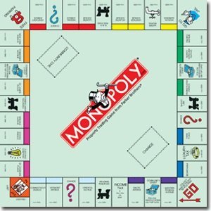Imagine you’re stuck in jail. On this turn, you can only get out if you roll doubles, i.e. both dice are showing the same outcome—2 + 2, 5 + 5, etc. Your friend has hotels on the oranges, so 3 + 3 and 4 + 4 are both bad news. If you land on free parking, 5 + 5, you get fat stacks of cash from the middle. Anything else is neutral.
This situation is a bit more complex than in blackjack, because now we have two dice, two random experiments, instead of just one card draw, governing our fate. Turns out, you can just create a sort of “bigger” random variable, which has an outcome space of die roll pairs, like (1,2) and (6,6), instead of just (1) or (3). Here are some possible input-output pairs from the random variable (there are 6 x 6 = 36 possible outcomes in Ω):

Outcome (die 1, die 2)	Value
(1,1)	$0 (electric company lol)
(1,2)	$0 (stuck in the slammer)
(3,3)	-$950 (st. james place)
(3,4)	$0 (stuck in the slammer)
(4,4)	-$950 (tennessee avenue)
(5,4)	$0 (stuck in the slammer)
(5,5)	+$1269 (free parking, big money)

Distribution of a Random Variable

Random variables do not tell us about the probability of these outcomes. We need a probability function for that. Without the handy random variable, we have to know specific outcomes of an experiment—the suit and number of my card, or the exact combination of my dice—to find their probability. But now, thanks to the handy random variable, given a probability function, we can ask what the probability of getting a specific value, not an outcome, is. Now we can completely ignore that other irrelevant stuff.

The distribution underlying a random variable simply tells us the probability of each value (again, bypassing clumsy outcomes, which when selected by randomness gods, determine the value of the random variable). Let’s look at the distributions underlying our earlier examples. The notation, Pr[ X=value ], tells us the probability that our random variable takes on this value. 

Example: Blackjack

52 cards, 4 cards per suit. Ace = 11.

X (the value of the random variable)	Pr[ X=value ]
11	1/13
10	4/13
9	1/13
2-8	7/13

Example: Monopoly

X (the value of the random variable)	Pr[ X=value ]
– $950	2/36 (land on hotels)
+ $1269	1/36 (land on free parking)
+ $0	33/36 (lucky doubles + stuck in slammer)

Hopefully this clears up some confusion regarding random variables and distributions. One of the hardest things for me when I took probability was getting accustomed to the notation and many unfamiliar terms getting thrown around. We’ll need this when I talk about entropy in my next post.

Food: This week, I made barbecue sauce! Slathered the stuff over bacon-chicken kebabs with peppers and onions, paired with a simple arugula salad, sweet potato fries, and pickled mustard seed.